Monthly Buy / Hold / Sell Recommendations
Dow Jones Industrial Average Index
Objective
In order to explore usage in R of machine learning and predictive packages:
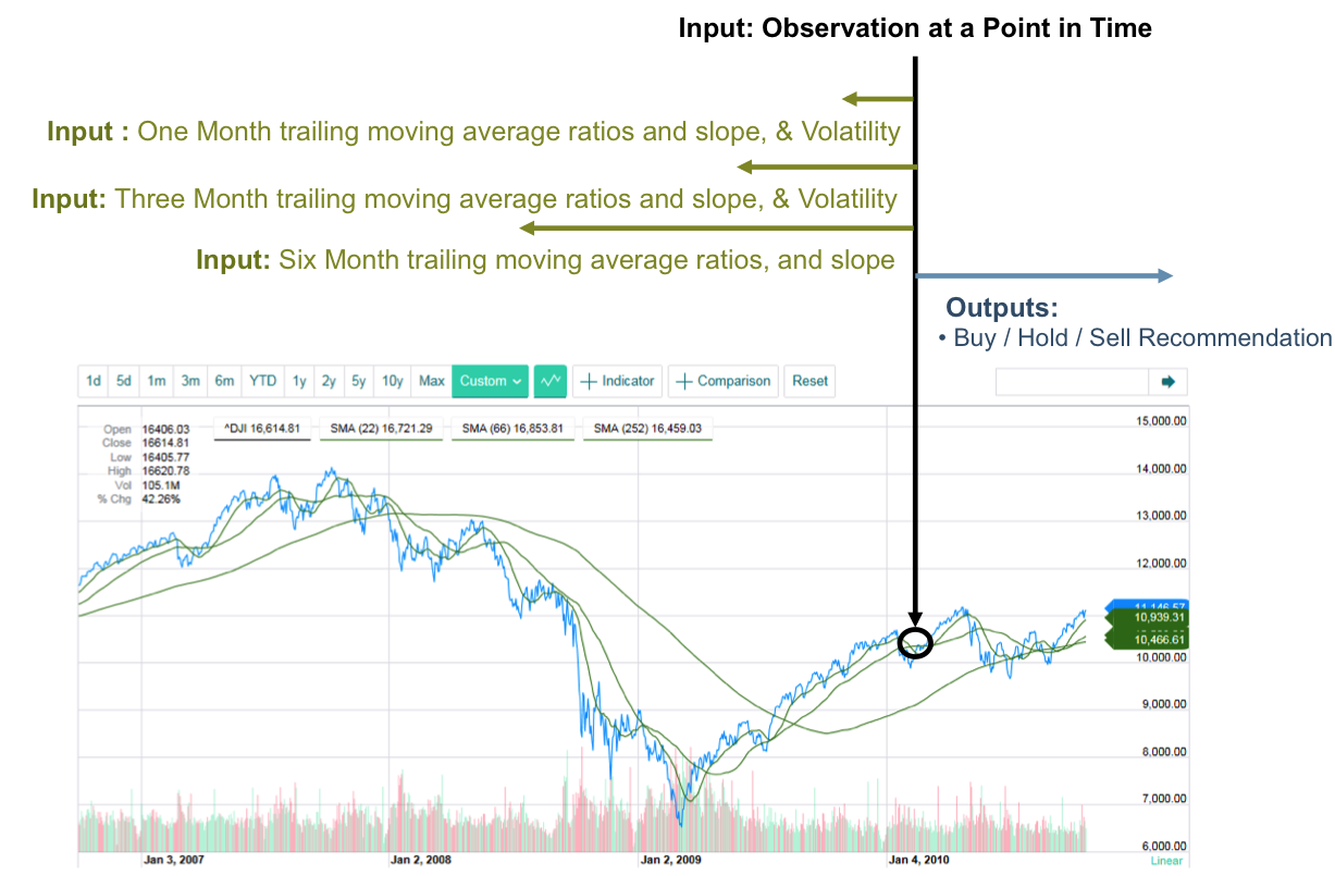
- Develop model that, for a specific observation of current indicators of the Dow Jones Industrial Average (DJIA) index, recommends whether to Buy / Hold / Sell DJIA index.
- The target audience is a Retail investor who may have restrictions in terms of frequent trading and should have longer time horizons in mind (i.e. no day trading) … hence the time horizon of the recommendation is in the order of Monthly /Quarterly.
Packages used: kmeans, C5.0, neuralnet
Background
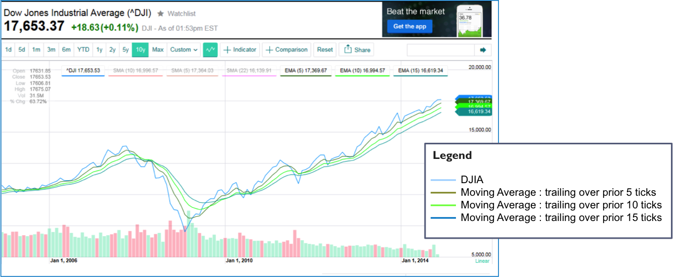
The chart below shows the closing price of the Dow Jones industrial average over the last decade:
We will use technical indicators (i.e. no macro economic indicators) with the assumption that the price history and pattern reflect the ‘crowd’s’ reaction, in terms of buying and selling, to geo-political and macro economic events. Another assumption is that the ‘crowd’s’ psychology does not significantly change over time, so that historical patterns in the price movement of the index reflect that ‘crowd’ psychology and hence can predict where the ‘crowd’ is going next
Key Indicators
Key Indicators used as inputs to the model:
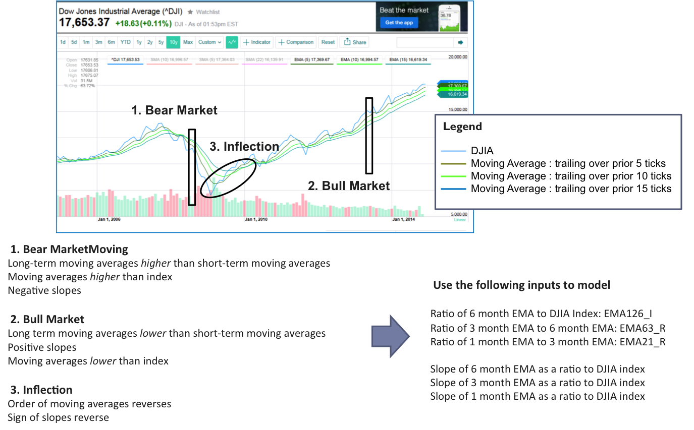
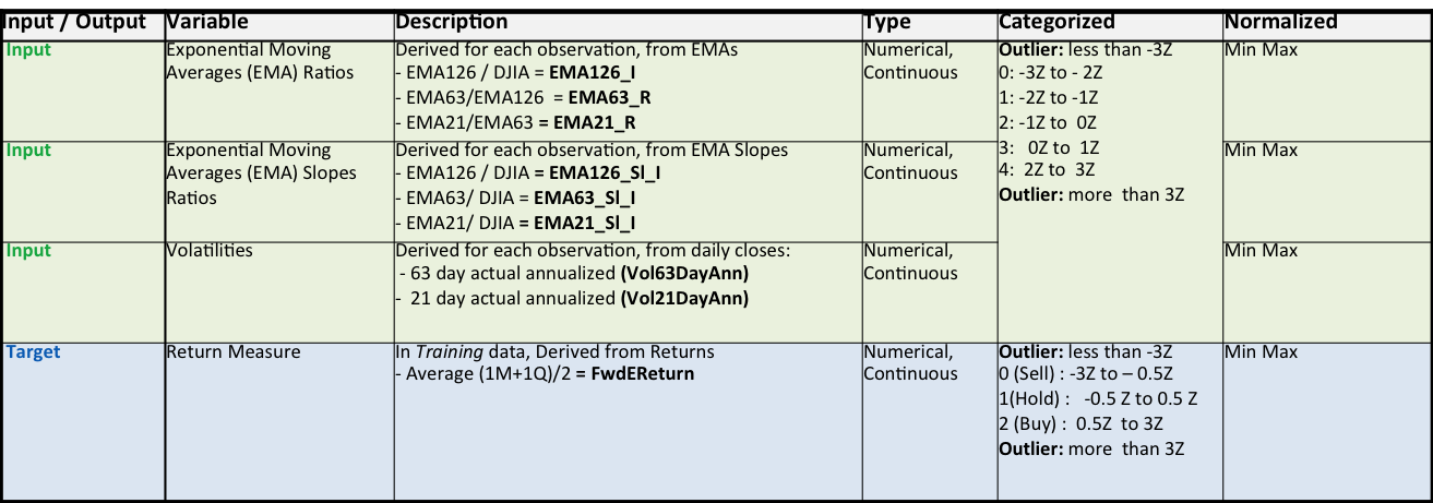
–Moving Averages, slopes and ratios among these – an indication of trends
-Observed Volatilities – an indication of fear or uncertainty
Output variable for machine learning:
-For training purposes, output variable – > observed forward Returns
This approach is (purposefully) different from traditional technical analysis -using indicators readily calculated from the time series – as opposed to techniques which use indicators such as support and breakout levels.
Moving Averages
- Help smooth the signal – and understand trend
- Reduce noise; However, “noise” is an important Indicator – see Volatility as a separate indicator
- Exponential moving averages (EMA) weigh recent observations more heavily so will be used instead of simple moving average
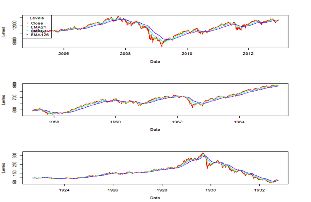
- From experience will use 21, 63 and 126 trading days as the Moving Average windows
Input and Output Variables
Sample R Snippets
Calculate EMAs ->
EMA21XTS<-EMA(closesXTS, n = 21)
Calculate EMA Indexes (i.e. ratio of EMA relative to actual Close)
djiaEMA$EMA126_I <- djiaEMA$EMA126/djia$Close
djiaEMA$EMA63_I <- djiaEMA$EMA63/djia$Close
djiaEMA$EMA21_I <- djiaEMA$EMA21/djia$Close
Calculate slope of 21 day exponential moving average->
djiaEMA<-data.frame(Date=index(djiaZEMA),djiaZEMA,row.names=NULL)
L<-length(djiaEMA$Close)
for (i in 31:L) {
djiaEMA$EMA21_Sl[i]=(as.numeric(djiaEMA$EMA21[i])-as.numeric(djiaEMA$EMA21[i-10]))/10
}
Plot EMAs and Slopes
par(mfrow=c(2,1))
tsRainbow <- rainbow(3)
plot(djiaZEMASl[32000:34000,c(15,16,17)], col = tsRainbow, screens=1, xlab =”Date”, ylab=”Levels”)
legend(“topleft”, title = “Levels”, col = tsRainbow, pch = 20, legend=c(names(djiaZEMASl[,c(15,16,17)])))
plot(djiaZEMASl[32000:34000,c(9,10,11)], col = tsRainbow, screens=1, xlab =”Date”, ylab=”Levels”)
legend(“topleft”, title = “Levels”, col = tsRainbow, pch = 20, legend=c(names(djiaZEMASl[,c(9,10,11)])))
Slopes
Models Used
kMeans Cluster
As part of the data understanding phase, run a kMeans Clustering analysis to understand whether it reveals any interesting patterns
Decision tree
- For efficiency, translated continuous inputs and target variable into categorical values
- Built decision tree with training data
- Tested with test data and tuned
- Used to predict results with validation data; Measured classification error rates
Neural Network
- To calculate Next Month’s predicted return
- Normalized inputs and target variables using Min Max (0 to 1)
- Measured prediction errors on testing set and validation set
Use of Models – Back Testing (not in scope for this project)
The true test of the models would be to back test the recommendations’ cumulative returns over a time period and compare those to the returns an investor would realize if the just ‘Held’ DJIA, which would be the control measure
Data Preparation
Sample raw data – >

Data categorized ->

Data min-max normalized ->
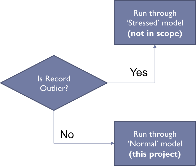
Outliers
Records with outliers in any of the input or target variables will be excluded
- Moving Averages
- Volatilities
- Returns
Z Scores used to detect outliers: < – 3Z or > 3Z
Outliers do not represent ‘incorrect’ data points, but times of extreme stress or euphoria in the markets. These would be modeled separately as these market events represent the greatest times of risk / opportunity (out of scope)
Sample R Snippets
Categorize by Z Score
L<-length(djia$Close)
myVarZ<- djia$FwdEReturnZ
myVarCat<- rep(0,L)
for (i in 1:L)
{
if (myVarZ[i]<(-3)){myVarCat[i]=0} else
{ if (myVarZ[i]<(-2)) {myVarCat[i]=1} else
{ if (myVarZ[i]<(-1)) {myVarCat[i]=2} else
{ if (myVarZ[i]<(0)) {myVarCat[i]=3} else
{ if (myVarZ[i]<(1)) {myVarCat[i]=4} else
{ if (myVarZ[i]<(2)) {myVarCat[i]=5} else
{ if (myVarZ[i]<(3)) {myVarCat[i]=6} else
{ myVarCat[i] = 7 }
}
}
}
}
}
}
}
djia$FwdEReturn_Cat<- rep(0,L)
djia$FwdEReturn_Cat<-myVarCat
Remove Outliers
myOutlierIndexFwdRet <- which(djia$FwdEReturnZ<(-3) | djia$FwdEReturnZ>(3))
djiaNoOutliers <- djia[-myOutlierIndex, ]
kMeans Clustering
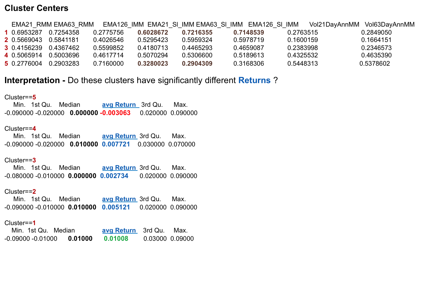
As part of the data understanding phase, I ran a kMeans Clustering analysis to understand whether it would reveal any interesting patterns. Used the R kmeans function with k = 5 on the entire monthly data set
Sample R Snippet
djiaKMeans<-djiaM[,c(“EMA21_RMM”,”EMA63_RMM”,”EMA126_IMM”,”EMA21_Sl_IMM”,”EMA63_Sl_IMM”,”EMA126_Sl_IMM”,”Vol21DayAnnMM”,”Vol63DayAnnMM”)]
km<-kmeans(djiaKMeans,centers=5)
Observations & Conclusions
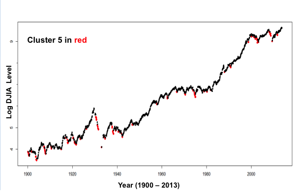
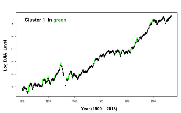
- Cluster ‘5’ corresponded to negative returns while Cluster 1 corresponded to the highest returns
- When plotted, Cluster ‘5’ corresponded to in many cases, sell signals, while Cluster 1 corresponded to in many cases to buy signals
Data points in Cluster 5 shown in Red –
plot(djiaM$Date,log(djiaM$Close),col=ifelse(djiaM$Clusters!=5,”black”,”red”),pch=ifelse(djiaM$Clusters==5,16,20))
Data points in Cluster 1 shown in Green –
plot(djiaM$Date,log(djiaM$Close),col=ifelse(djiaM$Clusters==1,”green”,”black”),pch=16)

The resulting k-centers may be used for new observations – i.e. observe which single cluster the new observation is closest to and from that categorize which market condition it belongs to. This could then be used to signal entry and exit points from the market – for example ‘3 consecutive green clusters signal entry, three consecutive red clusters signal exit, alternating red and green mean hold
Decision Tree
- Trained and tuned a set of decision trees using C50 (using the R C50 package)
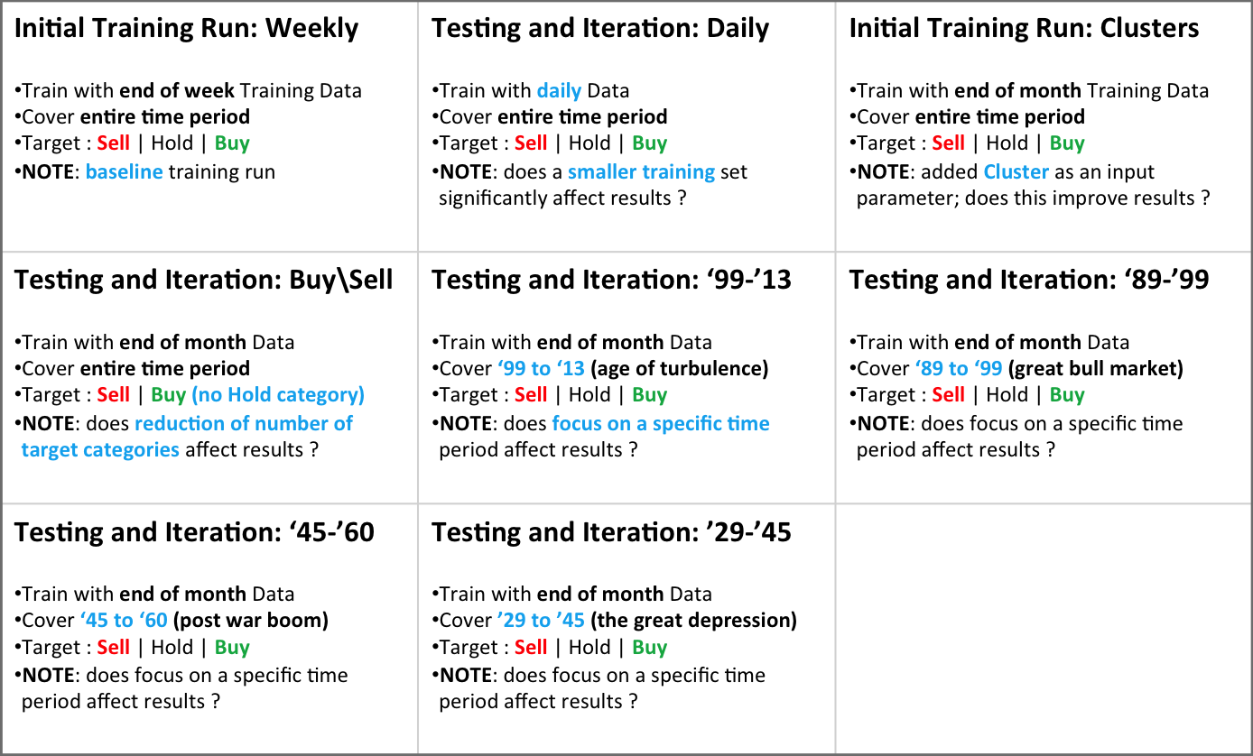
- Tried different time periods, training and test data sets, and classification schemes for target variable
- The chosen decision tree was used to predict Buy | Hold | Sell recommendations for the Validation data
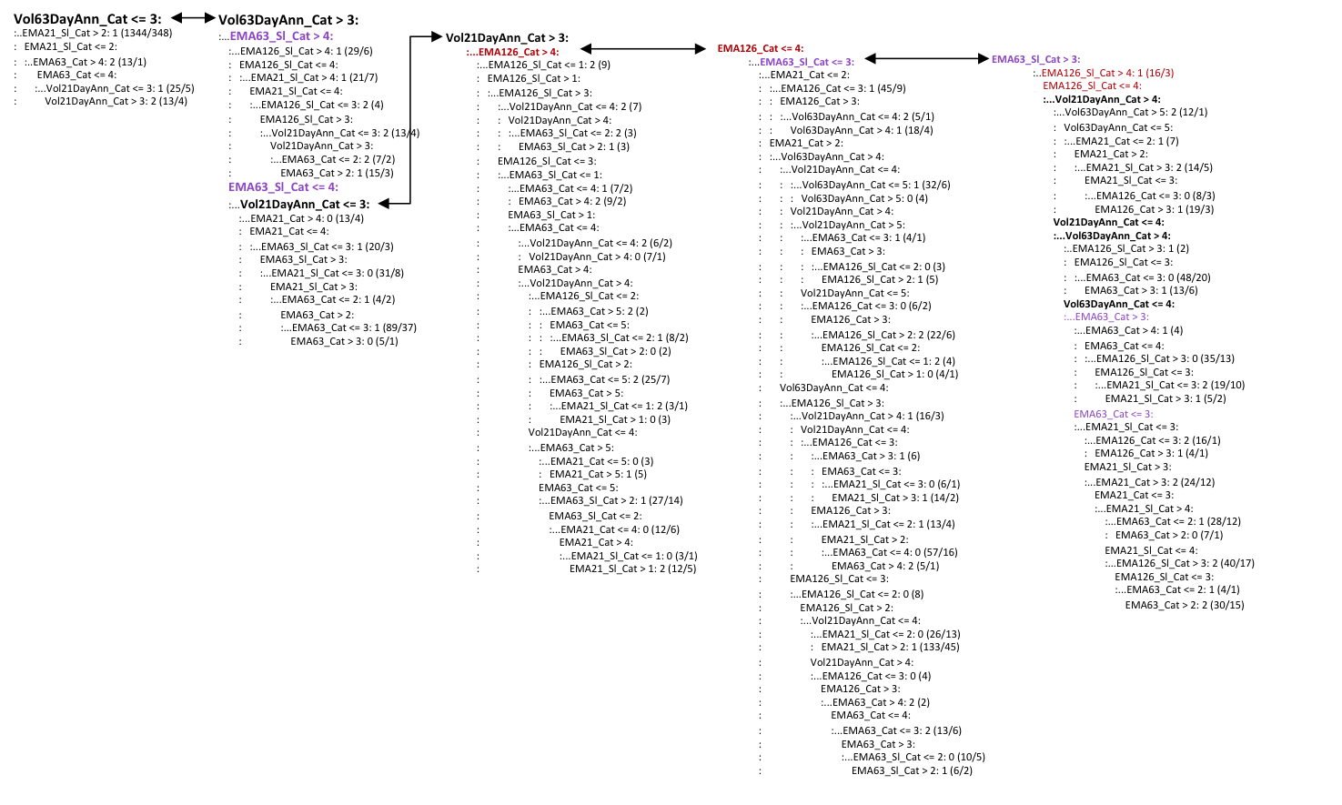
- A key finding in the tuning step was that the decision tree for each ‘era’ (e.g. ‘80’s vs. ‘30’s) was significantly different and of significantly different complexities. Even the most complex trees however were built quickly (within a second)
Sample R Snippets
Train Decision Tree
djiaRTInput<-djiaM[,c(“EMA21_Cat”,”EMA63_Cat”,”EMA126_Cat”,”EMA21_Sl_Cat”,”EMA63_Sl_Cat”,”EMA126_Sl_Cat”, “Vol21DayAnn_Cat”,”Vol63DayAnn_Cat”)]
djiaRTTrain<-factor(djiaM$FwdEReturn_CatS)
c50fit<-C5.0(djiaRTInput, djiaRTTrain)
summary(c50fit)
Attribute Usage — (for period 1999 – 2013)
- 100.00% Vol63Day
- 79.03% EMA21_Slope
- 46.92% EMA63_Slope
- 46.31% Vol21Day
- 37.37% EMA126_Index
- 36.42% EMA126_Slops
- 32.31% EMA21_Index
- 27.13% EMA63_Index\
Size (decision rule set ): 84
Error Rates:
- 28% on Training data
- 31% on Validation data
Predict with Resulting Decision Tree
valInData<-djiaM[,c(“EMA21_Cat”,”EMA63_Cat”,”EMA126_Cat”,”EMA21_Sl_Cat”,”EMA63_Sl_Cat”,”EMA126_Sl_Cat”, “Vol21DayAnn_Cat”,”Vol63DayAnn_Cat”)]
treeRecommend<-predict(c50fit,valInData,type=”class”)
Compare Predictions with Actuals
valOutData<-factor(djiaM$FwdReturn_CatS)
sum(treeRecommend == valOutData)/length(treeRecommend)
Tuning Iterations
- Larger (i.e. daily) training set resulted in more accurate decision tree
- Introducing Cluster simplified the decision tree but did not improve accuracy
- Simplifying the target variable categorization simplified the decision tree however reduced accuracy
- Each ‘era’ requires a different decision tree
- Attribute usage varies but the following appear to be the most important in most models: 63 day volatility, 126 day Index and slope
- Speed of prediction computations was within 1 second regardless of decision tree complexity
Results and Conclusions
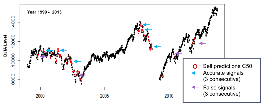
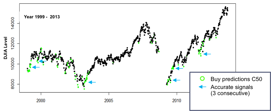
The 1999 – 2013 “era” data was used as input to the tuned decision tree to determine accuracy of predictions …
- Though a lower error rate is desirable, the decision tree made reasonably accurate predictions to buy or sell per the charts to the right, though there were some false buy / sell signals
- Similar to the kMeans cluster analysis, Buy / Sell decisions . should be made based on a series of consecutive consistent predictions from the model – for example ‘3 consecutive buy recommendations signal entry, three consecutive sell recommendations signal exit
- Bottoms seem to have conflicting Buy / Sell signals
Neural Network
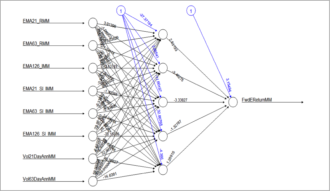
- The R package neuralnet was used
- Input parameters and target parameters, once outliers were extracted, were MinMax normalized
- Tested and iterated with testing data
- Ran and plotted results with validation data
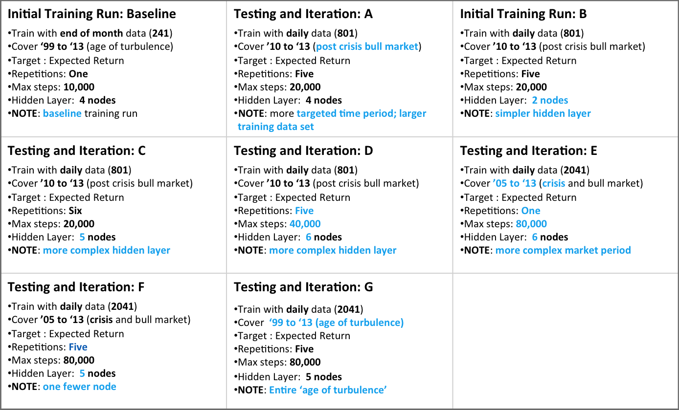
- Since the C50 results demonstrated that each ‘era’ has very different characteristics, I focused on modeling and validating the time period 1999 – 2013
Tuning Approach
Tried different runs, varying
- Time period of training data
- Number of neurons in hidden layer
- Number of repetitions for a specific configuration
- Max number of steps per repetition
Measured error rate as follows
- With weights resulting for a specific configuration of the model, predict forward returns with test data
- Measure / observe
- ¨Error rate and distribution of predictions – > Error % = (predicted value – actual value) / actual value
- ¨Distribution of predictions – > do these match distribution of actuals in terms of min / max / mean ?
Chose model with average lowest error %’s and prediction distribution closest to actual
Sample R Snippets
Train the Network with Training Data
library(neuralnet)
djiaNNInput <- djia[1152:1323,c(“EMA21_RMM”,”EMA63_RMM”,”EMA126_IMM”,”EMA21_Sl_IMM”,”EMA63_Sl_IMM”,”EMA126_Sl_IMM”, “Vol21DayAnnMM”,”Vol63DayAnnMM”,”FwdEReturnMM”)]
print(net.dat<-neuralnet(formula =
FwdEReturnMM~ EMA21_RMM + EMA63_RMM + EMA126_IMM
+ EMA21_Sl_IMM + EMA63_Sl_IMM + EMA126_Sl_IMM
+ Vol21DayAnnMM + Vol63DayAnnMM,
data=djiaNNDInput, rep = 1, hidden = 5, stepmax = 20000,
linear.output=FALSE))
plot(net.dat, rep = “best”)
Making predictions with generated neural network
djiaNNVal<- djiaV[1595:1835,c(“EMA21_RMM”,”EMA63_RMM”,”EMA126_IMM”,”EMA21_Sl_IMM”,”EMA63_Sl_IMM”,”EMA126_Sl_IMM”, “Vol21DayAnnMM”,”Vol63DayAnnMM”)]
NNtest<-compute(net.dat, djiaNNVal, rep = XBEST)
djiaV$NNPredict[1595:1835]<- NNtest$net.result
Preliminary Results
The neural network shown above was chosen from different configurations tested with test data. It was trained with training data from a daily set of observations from 1999 through 2013
The validation data was then input to the NN and predictions computed
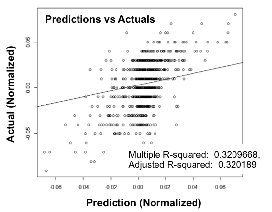
The predictions were plotted against the actuals on the plot and a best fit line drawn
If the predictions are 100 % accurate we would see a diagonal straight line. The plot does not show a very close correlation of predicted to actual.
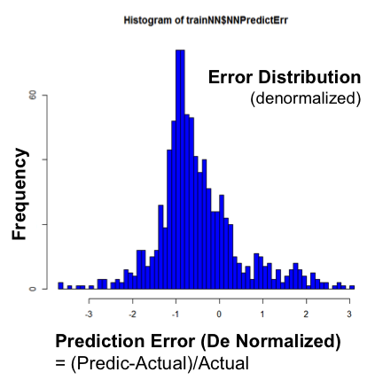
The errors were then computed across the validation data and plotted on the histogram on the right
Error = (PredictedReturn / Actual Return) / ActualReturn
The histogram shows significant levels of errors, tending to underestimate the actual
Preliminary Conclusion ; this NN does not accurately predict expected results. HOWEVER I next looked at the results in a different way ->
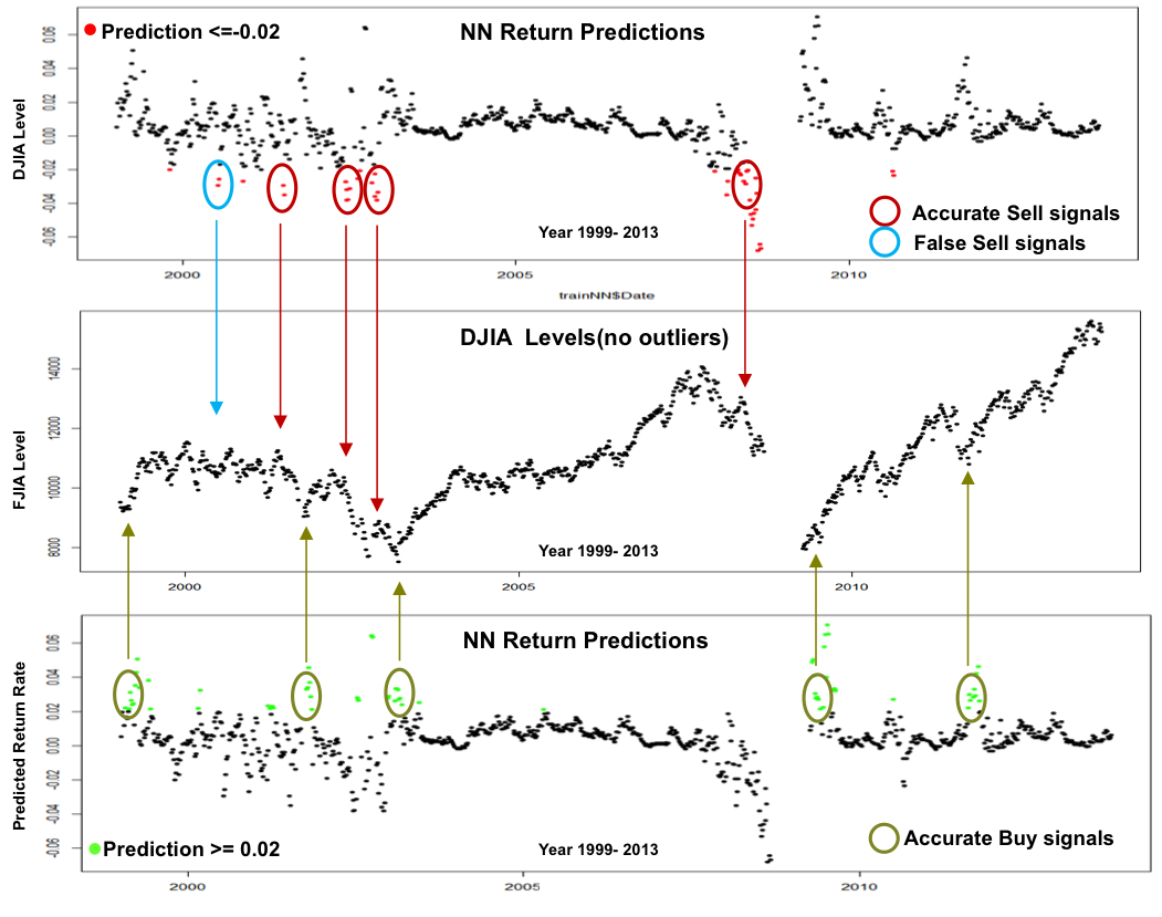
Interpreting NN Results As Signals
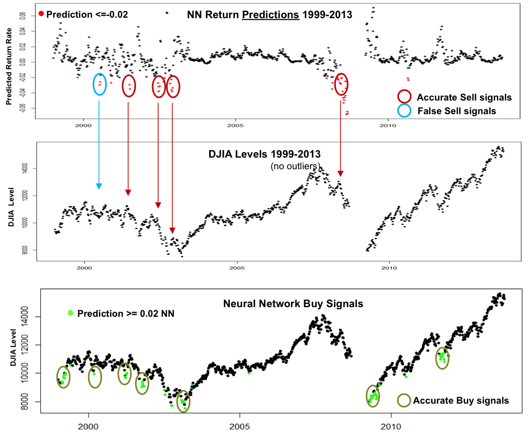
Since the actual Return predictions of the NN proved disappointing, the predicted Returns were plotted as time series to confirm how they related to the actual DJIA index
The plot on the top has predicted results and in Red highlights those that are less than 0.02.
The plot on the bottom has predicted results and in Green highlights those that higher than 0.02.
The plots below illustrate this
Conclusions
Setting Predicted Return <= 0.02 as a a Buy Signal generated fairly accurate signals, especially if the signals occur in sequence over a small period of time
Setting Predicted Return <= -0.02 as a Sell signal generated mostly accurate Sell signals, especially if the signals occur in sequence over a small period of time
The shape of the predictions plot compared to the DJIA plot shows promise – further tuning may yield better predictions
Overall Conclusions
- C50 did a reasonable job of raising Sell and Buy signals, better with Buys
- NN did not do a good job of predicting returns but did better in raising Buy / Sell signals – especially Buy signals
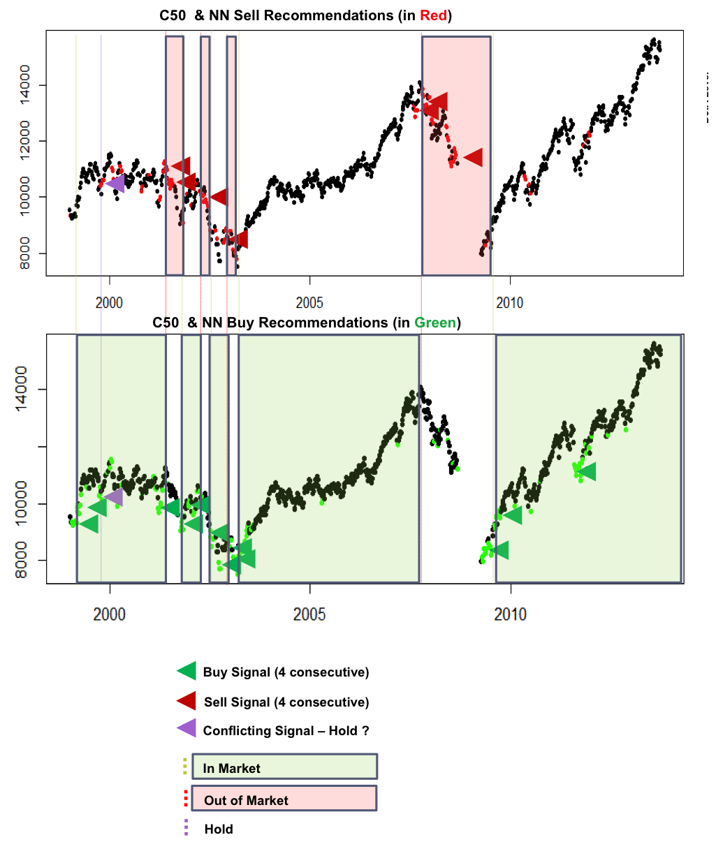
- The charts below show a different view of the signals. The C50 and NN Sell and Buy signals are shown in one plot, and Signals identified when there are 4 or more consecutive consistent predictions
- Based on these signals, entry and exit points are shown, with shaded areas for signals to be In the market and Out of the market
- The combination of models make a very good job of identifying when to be in the market and when to be out
Next Steps
So am I now sipping margaritas and retired in my private Tahitian Island? Unfortunately not. I briefly used the models on recent market data with mixed results. Why ? I probably overtrained the models, but I think they show promise ; )
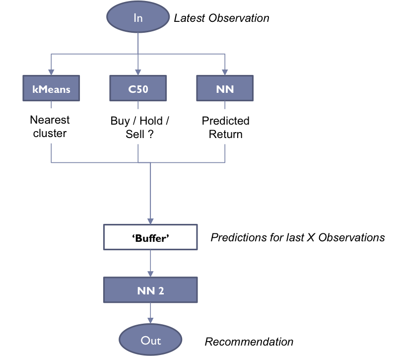
- Create a predictive model that takes in as input a series of signals from the other models to trigger an entry or exit from the market
- Back test the model
Check out the project here : Class 637 Project Submission Fall 2014 v3

